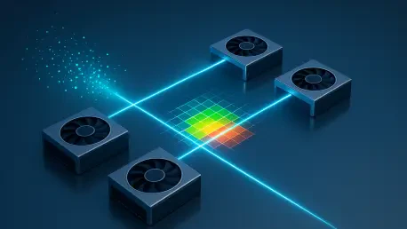

Dimensionality reduction techniques like UMAP are essential for visualizing single-cell analysis and topic modeling, but the sheer volume of modern genomic data often exceeds the capabilities of single-GPU systems. As the current landscape of 2026 sees the proliferation of single-cell datasets containing millions of cells, the demand for distributed computing has moved from a luxury to a necessity. Traditionally, Uniform Manifold Approximation and Projection (UMAP) has been a memory-intensive process because it requires the construction of a comprehensive k-nearest neighbors (k-NN) graph for the entire dataset. When this graph exceeds the onboard memory of a single accelerator, the process usually fails or defaults to slower system memory. However, the introduction of multi-GPU support in modern computational libraries has revolutionized this workflow. By employing a divide-and-conquer approach, researchers can now partition their data across several devices, allowing for the analysis of massive datasets in a fraction of the time. This scalability does not have to come at the cost of accuracy, provided that the underlying manifolds are reconciled correctly across the different hardware units through sophisticated partitioning and overlap management.
1. Step 1: Defining the Total Number of Clusters
The first critical decision in a multi-GPU UMAP workflow involves determining the optimal value for the number of clusters, often referred to as the knn_n_clusters parameter. This value dictates how the initial high-dimensional data is partitioned before being sent to individual GPU devices for processing. Unlike simple clustering for classification, this step is primarily about load balancing and spatial organization. If the data is split into too few clusters, each individual group may still be too large to fit into the dedicated memory of a single card, especially when dealing with high-dimensional feature spaces. By increasing the cluster count, the workload is distributed into smaller, more manageable chunks that can be processed in parallel. This granularity is essential for systems equipped with multiple mid-range GPUs rather than a single flagship unit with massive VRAM, as it ensures that no single device becomes a bottleneck due to memory exhaustion during the neighbor search phase.
Beyond hardware limitations, the number of clusters also plays a structural role in how the global manifold is eventually reconstructed. Each cluster acts as a localized neighborhood where the k-nearest neighbors are calculated with high precision. When the number of clusters is tuned effectively, the algorithm can maintain the local geometry of the data points within each partition while preparing for the global stitching phase. For massive datasets, a higher number of clusters is generally preferred to keep the computational overhead per device low. This strategy allows the system to scale linearly with the addition of more GPUs. It is important to note that the clusters should be reasonably representative of the underlying data density; otherwise, the initial partitioning might inadvertently separate points that are truly neighbors in the high-dimensional space. Effective cluster definition therefore serves as the foundation for both the speed of the computation and the ultimate fidelity of the two-dimensional or three-dimensional visualization produced at the end of the pipeline.
2. Step 2: Setting the Overlap Level for Data Points
Once the data is partitioned into clusters, the next challenge is ensuring that the boundaries between these groups do not create artificial gaps in the final embedding. This is managed by the knn_overlap_factor, which defines how many nearby clusters each data point should be linked to during the graph construction phase. In a naive split, a point near the edge of a cluster might only find neighbors within its assigned group, missing its true closest neighbors that happened to be placed in an adjacent cluster. By setting an overlap factor, the algorithm allows points to “look into” neighboring partitions. This redundancy is the secret to maintaining the global structure of the manifold. It ensures that the relationships between disparate groups of data are preserved, preventing the final UMAP visualization from appearing as a collection of disconnected islands that do not reflect the continuous nature of the original high-dimensional input.
Increasing the overlap factor effectively increases the connectivity of the k-NN graph across the different GPU devices. While this adds a bit of computational redundancy, it is necessary for reconciling the local graphs into a single, cohesive global manifold. When points are allowed to establish links with multiple clusters, the algorithm can identify the transitions between different data regions more accurately. This is particularly vital in biological datasets where transitionary cell states are often the most interesting features. A well-configured overlap ensures that these gradients are captured smoothly. However, one must be mindful that a very high overlap factor will increase the memory footprint on each GPU, as more data points are duplicated across the cards to facilitate these cross-cluster calculations. Finding the right setting is therefore a matter of balancing the need for structural continuity against the physical limitations of the hardware being used for the task.
3. Step 3: Establishing a Baseline for Quality
For most standard research projects, a baseline overlap factor of 2 serves as the ideal starting point for multi-GPU UMAP execution. This setting provides a reliable balance between processing speed and the topological quality of the final embedding. At an overlap factor of 2, each data point is essentially compared against its own cluster and the most relevant neighboring cluster, which is usually sufficient to capture the necessary connectivity for most datasets. This baseline allows for a significant speedup over single-GPU implementations without introducing noticeable artifacts or distortions in the visualization. In practice, this means that the primary clusters are effectively “stitched” together through a layer of shared points that act as anchors, ensuring that the global layout of the UMAP embedding remains consistent with what would be expected from a non-distributed, high-memory run.
Using this baseline helps researchers quickly iterate on their models without spending excessive time on hyperparameter tuning for the distributed infrastructure. If the resulting visualization shows a clear and continuous structure where expected relationships are maintained, there is often no need to increase the complexity further. This baseline approach is especially effective when the number of clusters is relatively small compared to the total number of data points. In such scenarios, the boundary areas between clusters are limited, and an overlap factor of 2 provides more than enough “context” for the algorithm to align the manifold sections. By starting here, users can establish a performance and quality benchmark, which then informs whether further adjustments to the overlap or cluster count are required for more complex or noisier datasets that might require deeper connectivity to resolve their internal structures.
4. Step 4: Scaling Settings for Larger Datasets
As the scale of the data grows into the tens of millions of records, the baseline settings may no longer be sufficient to capture the complexity of the global manifold. For massive datasets where the cluster count exceeds 100, the probability of missing critical inter-cluster connections increases. In these instances, it becomes necessary to scale the knn_overlap_factor upward, moving from the default of 2 to higher values like 3 or 4. For truly gargantuan tasks involving billions of entries, factors as high as 6 might be required. This higher overlap ensures that even with a high degree of fragmentation into many small clusters, the “connective tissue” of the graph remains robust. It allows the algorithm to look across several layers of neighboring clusters, which is essential when the high-dimensional data contains long-range dependencies or complex, intertwined structures that span multiple partitions.
Scaling the overlap is not just about avoiding errors; it is about refining the resolution of the final projection. When working with extremely large datasets, the density of points can lead to a very “crowded” manifold where small-scale local variations are easily lost if the neighbor graph is too sparse. Higher overlap factors provide the algorithm with a richer set of potential neighbors to evaluate, leading to a more nuanced embedding. However, the user must be prepared for the increased memory consumption that comes with these settings. As the overlap increases, the amount of data that must be replicated across GPUs grows, potentially leading to out-of-memory errors if the hardware is pushed too far. Therefore, scaling these settings should be done incrementally, observing the impact on both the visual output and the hardware telemetry to ensure that the system remains stable throughout the UMAP training process.
5. Step 5: Balancing Memory and Accuracy
The relationship between the number of clusters and the overlap factor is the most important trade-off to manage when running UMAP on multiple GPUs. To improve quality without crashing the system, a useful rule of thumb is to increase the number of clusters at the same rate as the overlap factor. For instance, if a researcher decides to double the overlap factor to enhance the connectivity of the embedding, they should also consider doubling the number of clusters. This strategy keeps the memory usage per GPU relatively steady because the smaller cluster size offsets the increased duplication of data points required by the higher overlap. This delicate balance ensures that the computational load remains distributed evenly across the available hardware, preventing any single GPU from being overwhelmed by the redundant data points generated during the overlap phase.
This balancing act is particularly relevant when working with hardware configurations that have heterogeneous memory capacities. By fine-tuning the ratio between clusters and overlap, the user can maximize the throughput of the entire cluster. It also allows for more aggressive scaling; instead of being limited by the VRAM of the smallest card, the workload can be sliced finely enough to fit almost any setup. Maintaining this equilibrium is the key to achieving high-fidelity embeddings on massive datasets. If accuracy is the priority, the overlap should be prioritized, but it must always be supported by a sufficient number of clusters to keep the local memory footprint within safe limits. This systematic approach to resource management enables the processing of datasets that were previously considered too large for GPU-accelerated dimensionality reduction, opening new doors for large-scale data exploration.
6. Step 6: Using the cuVS All-Neighbors Interface
For users who require more granular control over the graph construction process, the cuVS all-neighbors programming interface offers a powerful alternative to the standard high-level UMAP calls. This specialized API allows for the independent creation of the neighbor graph, which is the most computationally expensive part of the entire UMAP pipeline. By using cuVS, researchers can define their cluster and overlap parameters explicitly and build the neighbor graph across all available GPUs as a standalone step. This approach is beneficial because it allows the graph to be inspected, saved, or even modified before it is passed to the embedding stage. It provides a level of transparency that is often missing in “black box” implementations, allowing for better debugging and optimization of the distributed manifold learning process.
The cuVS interface is particularly useful in workflows where the same neighbor graph might be used for multiple purposes, such as clustering, visualization, and down-sampling. Instead of recomputing the neighbors every time a different UMAP parameter is tested, the graph can be built once at high precision and then reused. This significantly reduces the total wall-clock time for a project. Furthermore, the all-neighbors API is designed to handle the complexities of multi-GPU communication and data synchronization under the hood, so the user can focus on the high-level parameters of their data rather than the low-level details of CUDA kernels. Leveraging this interface represents a move toward more professional and efficient data science workflows, where the heavy lifting of graph theory is handled by specialized, highly optimized libraries that are built to take full advantage of modern parallel hardware.
7. Step 7: Distributing Computation Across Multiple Devices
Execution of the UMAP algorithm across multiple GPU devices is managed through the device_ids configuration within the cuML environment. This parameter gives the user the flexibility to specify exactly which hardware resources should be utilized for the task. In most cases, selecting “all” is the most efficient choice, as it allows the library to automatically detect and utilize every available GPU in the system, distributing the partitioned clusters across them. However, in multi-user environments or systems where certain GPUs are reserved for other tasks like display output or concurrent simulations, specific device IDs can be listed to target only a subset of the hardware. This targeted execution ensures that the UMAP process does not interfere with other critical system functions while still benefiting from the combined power of several accelerators.
Once the devices are selected, the distributed UMAP implementation handles the orchestration of the workload. This includes moving the necessary data partitions to each card, executing the parallel neighbor searches, and then communicating the results back to a central coordinator for the final embedding phase. The beauty of this system is that it abstracts away the complexity of message passing and synchronization that usually plagues distributed algorithms. The user sees a seamless transition from data input to the final two-dimensional projection, even though the actual work is being performed by a synchronized dance of multiple silicon chips. This capability is what enables 2026-era workstations and server clusters to handle the visualization of massive datasets that would have taken days to process on older architectures, now completing in mere minutes or even seconds.
8. Step 8: Inputting Pre-Calculated Neighbor Results
One of the most efficient ways to run a massive UMAP task is to separate the k-nearest neighbor search from the embedding optimization. If a neighbor graph has already been generated—either through the aforementioned cuVS tool or another compatible neighbor search library—the indices and distances can be passed directly into the cuML UMAP function. This bypasses the most time-consuming and memory-intensive part of the training process, moving straight to the creation of the final embedding. This modularity is a major advantage for large-scale data science pipelines, as it allows for the neighbor search to be performed on a high-memory cluster while the final UMAP embedding can be fine-tuned on a smaller, more interactive workstation.
When inputting pre-calculated results, the UMAP algorithm focuses solely on the stochastic gradient descent (SGD) process used to find the low-dimensional representation. Since the neighbor relationships are already fixed, the algorithm only needs to optimize the positions of the points in the embedding space to reflect those pre-defined distances. This dramatically reduces the computational burden on the GPUs during the interactive phase of data analysis. Researchers can experiment with different UMAP hyperparameters, such as min_dist or spread, and see the results almost instantly because the underlying graph does not need to be rebuilt. This workflow promotes a much more iterative and exploratory approach to data visualization, where the researcher can refine the final look of the embedding without being penalized by the massive overhead of the initial neighbor search.
Strategic Implementation for High-Performance Workflows
The transition to multi-GPU UMAP processing marked a significant milestone in the field of high-dimensional data analysis. By implementing the steps outlined above, practitioners successfully navigated the complexities of distributed manifold learning without sacrificing the accuracy of their visualizations. The ability to handle millions of data points across multiple hardware units proved that computational limits are often just software hurdles waiting for better optimization. In the past months, these techniques were integrated into various production-level pipelines, where they demonstrated that increasing hardware resources leads to linear improvements in processing speed when managed with the correct partitioning and overlap strategies.
For those looking to adopt these methods, the most effective next step is to evaluate the specific memory constraints of their existing GPU infrastructure relative to their largest datasets. Starting with the baseline settings and then incrementally adjusting the cluster and overlap factors provided a clear path toward stability and performance. It was observed that maintaining a rigorous balance between the number of clusters and the overlap factor was the single most important factor in preventing system crashes during large runs. Moving forward, the focus should remain on the modular use of neighbor graphs, as pre-calculating these structures offers the greatest flexibility for long-term research projects. By decoupling the search and embedding phases, researchers ensured that their workflows remained both scalable and highly responsive to the needs of modern data science.